Download and Save Analytics Template

Each analytics template will be listed in the Help portal by template.  Open the Template topic, and then click the link to download the template to your computer or network.

Export Report Data and Load in Template

1.     Specify the report parameters according the selected template instructions. Specify the reporting interval, grouping and filter options.

•        Note: Select the group level that provides the best relative comparisons.

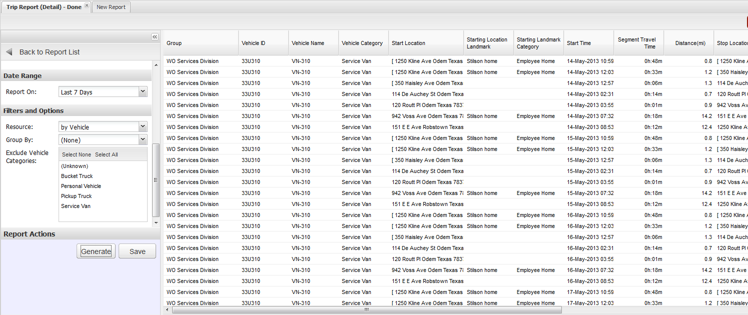
2.     Export to CSV format. Select the HH:MM:SS  format option.

3.     Open the exported CSV report in Excel.

4.     Copy the data by selecting all the data except the top row.  Select the cells only, not the entire row. Your selected cells should include columns A through column AD.  The cell range will look like A2:ADxxx where xxx indicates the rows of data.

5.     Paste the copied data into the appropriate tab on the Anayltics template.

Populate the Analytics Template

1.     Open the Analytics Template and select the Paste [Name of Template] Here tab.

2.     Select the top-left cell located below the column headers. This is typically cell C7 or C8.

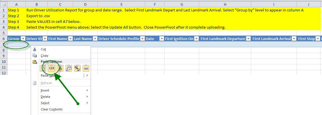
3.     Right-click and select the Values paste button from the short-cut menu.

4.     If you are adding rows of data to an already existing template, past the values in the next open cell in column A.

Update PowerPivot

The next step is to update the PowerPivot OLAP database with the data pasted. The PowerPivot tool attached to an Excel file is an OLAP database. For more information on OLAP databse, refer to Analytics Overview.

1.     From the Excel ribbon, select the PowerPivot tab.

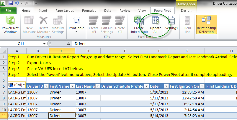
2.     Click the Update All button.

•        PowerPivot will take several minutes to update the database.

3.     When the upload is complete, close the window.

Update Analytics

1.     Select the Analytics tab, and select the cell or chart block as instructed at the top of each tab.

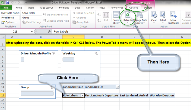
•        For example,  the top of the Analytics tab reads "select Cell C13."

•        When you select the appropriate cell, Excel displays the PivotTable Tools on the ribbon. The PivotTable Tools ribbon has two tabs: Options and Design.

•        When you select the chart block, Excel displays the PivotChart Tools on the ribbon. The PivotChart Tools ribbon has four tabs: Design, Layout, Format and Analyze.

2.     Select the Options tab, and then click the Refresh button.

3.     To update charts, select the chart block. Then, select the Analyze tab, and then click the Refresh button.

4.     For each tab, repeat the above steps to update the data.